It can be in the same worksheet or another one. Find the Format As Table.
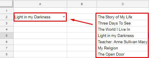
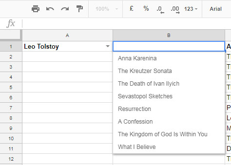
Multi Row Dynamic Dependent Drop Down List In Google Sheets
Click OK then in the PivotTable Fields pane drag the column you want to create drop down list based on to the Rows section.

How to make drop down list in excel table. Select List from field Allow and within the Source field write the new name of the table with as a prefix. Go to the Data tab on the Ribbon then click Data Validation. When you get to the step 5.
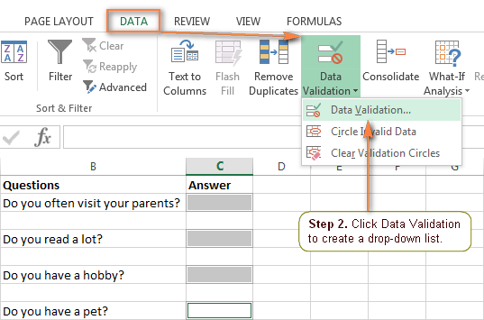
PivotTable then choose a position for the new PivotTable. Next navigate to Data tab in the Excel Ribbon and then click the Data Validation button. Go to Data.
On the Settings tab in the Allow box click List. Drop-down list with data lookup in Excel. 09042021 To make your primary drop-down list configure an Excel Data Validation rule in this way.
Select the table click Insert. In Settings tab select List in the drop down and in Source field select the unique list of countries that we generated. Highlight the range for the drop-down list.
TableNameColumn If you are not sure show a screenshot of the excel Table. It is necessary to make a drop-down list with values from the dynamic range. 22012021 Enter the data you want to appear in the drop-down list.
Now click OK and youre are done. Click the Source box select your list. Select a cell in which you want the dropdown to appear D3 in our case.
Select the cell where you want the drop-down list to appear and then select Data. Create a data validation rule for the dependent dropdown list with a custom formula based on the INDIRECT function. On the Data tab in the Data Tools group click Data Validation.
Check the Excel Essentials Course. Now a Data Validation window will open. Tool in the main menu.
Under Allow select List. How to make a drop down list in Excel. 27082020 Select E4 in the new sheet and repeat the instructions for creating a drop down from a previous Excel article through step 4.
In the Data Validation dialog box do the following. If changes are made to the available range data are added or deleted they are automatically reflected in the drop-down list. 22022017 Now select the cell you want to apply the dynamic dropdown menu to and go to DATA.
For the detailed steps please see Making a drop down list based on a named range. However do not include the header cell. 02022014 Here are the steps to create a drop down list in a cell.
If you already made a table with the drop-down entries click in the Source box and then click and drag the cells that contain those entries. INDIRECTB5 In this formula INDIRECT simply evaluates values in column B as references which links them to the named ranges previously defined. 31082020 If your Excel Table has powerAppId and you have already connected to the App on the Items property of the Dropdown put.
In Data Validation dialogue box select the Settings tab. 29082019 Go to the Data tab click Data Validation and set up a drop-down list based on a named range in the usual way by selecting List under Allow and entering the range name in the Source box. First of all open your excel sheet and select the cell on which you wish to create a drop down.
How To Add A Drop Down Box In Excel 2007 11 Steps With Pictures

How To Create Drop Down Lists In Excel Complete Guide Video Tutorial

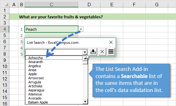
How To Search Data Validation Drop Down Lists In Excel Excel Campus
Drop Down List In Excel In 2020 Data Validation Excel Tutorials Excel Shortcuts

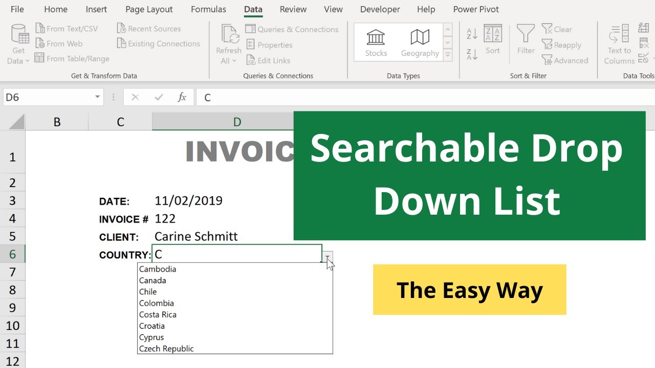
Searchable Drop Down List In Excel The Easy Way Youtube
How To Create Yes Or No Drop Down List With Color In Excel

Multi Row Dynamic Dependent Drop Down List In Google Sheets
Cara Membuat Drop Down List Di Excel Dengan Cepat Kiatexcel Com

Excel Drop Down List How To Create Edit And Remove Data Validation Lists


0 comments:
Post a Comment