26102010 Change Allow to List Source to the data you want the source to be Click and select But this only creates a drop down list in a cell with the data you selected as options it doesnt filter or anything. Create from Selection see screenshot.

How To Create A Drop Down List In Excel The Only Guide You Need
Just kidding but youve made great strides today.
How to create drop down list in excel header. 25112014 Here are the steps to create the icon. Select List from the Allow. Now your data wont get messy ever again.
Then select the first drop down list values excluding the header cell and then give a range name for them in the Name box which besides the formula bar see screenshot. The Data Validation dialog box displays. Then in the Source selector click and drag across cell D2D5 you dont want you folks to be able to choose the data header.
Create a new header in column D1 titled Location and name column E1 Surgeons. On the Settings tab in the Allow box click List. To use the drop down.
On the Excel ribbon go to the Data tab. After you add letter headings to the product list its easy to get to any part of the list. Type a letter in the cell.
In the drop-down under Allow choose List. 27012021 From the top of the page click Data to switch tabs. And then select the second drop down list data and then click Formulas.
On the Symbol window choose Wingdings 3 from the Text drop-down. On the Data ribbon Select Data Validation. Click the arrow next to Total and sort by largest to smallest or smallest to largest by clicking the appropriate option in the dropdown.
11052020 I drag this formula down column E so that I see this value in January February March etc. 26032018 Use Excel Data Validation to create a drop-down list. Select the cell to the right of the cell that contains a validation list.
Column E with a drop down list of currencies Column F with a drop down list of currencies and Column G with the formula inserted to divide the value in column E by column F. Enter the list. Data Tools group and click Data Validation.
Type a single letter in the cell then click the drop down arrow. No macros are needed to use the drop down list with letter headings. On the sheet to have the DropDowns select cell A2.
If you want to filter just select the header row and do Data. 22042020 First return to the wks spreadsheet and delete the previous drop-down list in column D titled Surgeons. Click the drop down arrow to open the list.
29082019 Go to the Data tab click Data Validation and set up a drop-down list based on a named range in the usual way by selecting List under Allow and entering the range name in the Source box. I figure this process could be simplified by creating three new columns. However do not include the header cell.
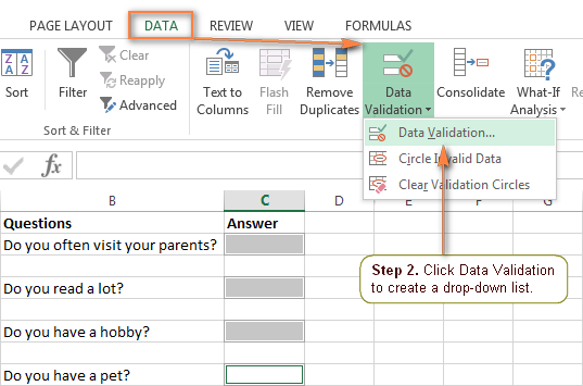
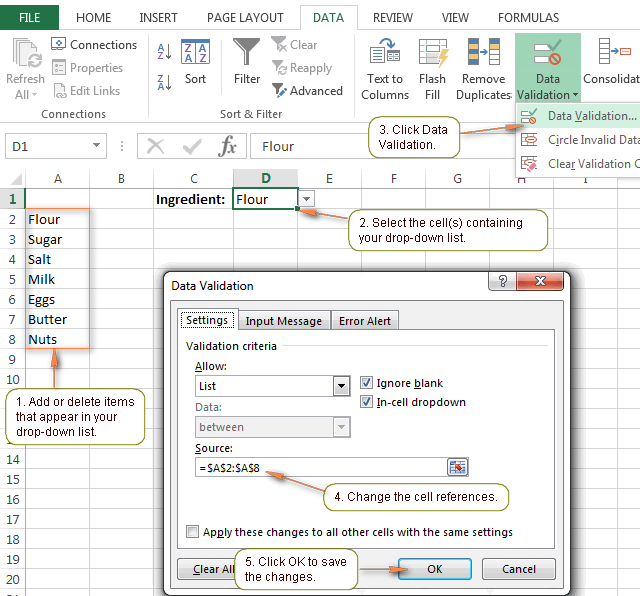
24012017 Now select the cell into which you want to add a drop-down list and click the Data tab. On the Settings tab select List from the Allow drop-down list see drop-down lists are everywhere. Enter the title of.
Go to the Insert tab on the ribbon press the Symbol button. If you already made a table with the drop-down entries click in the Source box and then click and drag the cells that contain those entries. Youre so close Check it out you created a drop-down list.
For the detailed steps please see Making a drop down list based on a named range. The list opens at the letter you typed so you can quickly find the item you need. 15092018 Enter the required headers in row 1 of Sheet1.
Enter the following formula in the Source field OFFSETSheet1A1001COUNTASheet111-COLUMN1 Copy cell A2 to cells to the right for as many as required. This will add a small down arrow to the right of each heading. To set up the letter headings.
Add the letter headings manually. Either choose Insert Column Right or Insert Column Left A new tab will pop up. Go to the Data tab on the Ribbon then click Data Validation.
In the Data Tools section of the Data tab click the Data Validation button. 18052021 Click on the three-dot icon on the column header where you want to add a new dropdown list. 21012021 On another sheet the MyList named range is used as the source for a data validation drop down.
Filter then click the Filter icon.
How To Create A Drop Down List With Dynamic Content How To Excel
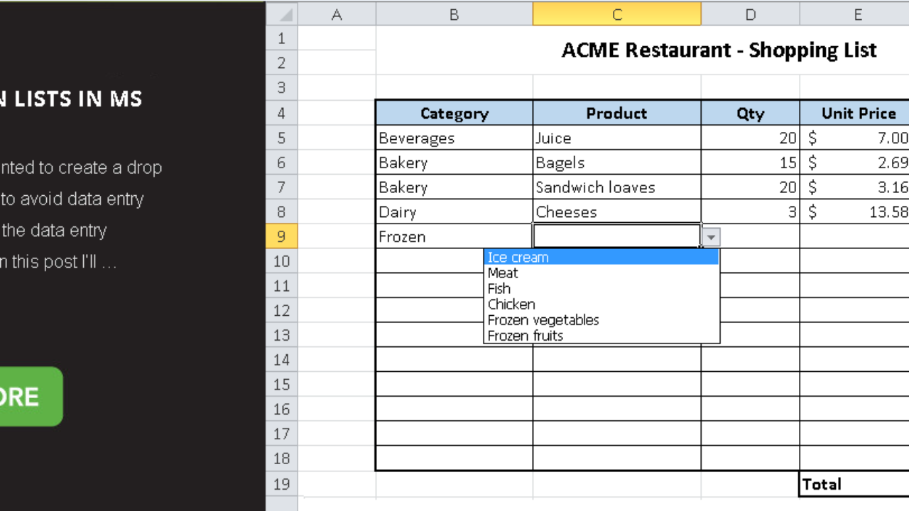
How To Work With Drop Down Lists In Ms Excel Master Data Analysis

How To Create Yes Or No Drop Down List With Color In Excel
Excel Drop Down List How To Create Edit And Remove Data Validation Lists
Excel Drop Down List How To Create Edit And Remove Data Validation Lists

How To Add A Drop Down Box In Excel 2007 11 Steps With Pictures
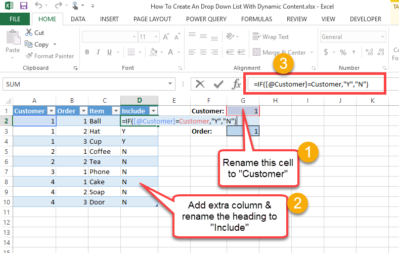
How To Create A Drop Down List With Dynamic Content How To Excel
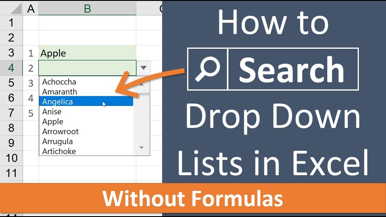
How To Search Data Validation Drop Down Lists In Excel Excel Campus

How To Create A Drop Down List In Excel With Examples Magoosh Excel Blog


0 comments:
Post a Comment