Colored Drop-down List see screenshot. Tab then click the Styles.

How To Add Color To Drop Down List In Excel
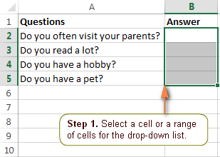
First you should create the drop down list that you want to use see screenshot.
How to make a drop down list in excel that changes color. Now our table now has conditional formatting applied. For the Source highlight what the choices you want to be found in your dropdown list. And then click the OK button.
12112019 Create a Drop Down list. 28082020 To begin add a new sheet and then add a new list with the text items red blue green and yellow Figure A. A dropdown list will be created on the cell.
Click OK twice to return to the Conditional Formatting Rules Manager. 2 Add colors to the items of drop-down list one by one. 01102020 Mark the desired column that should contain the color dropdowns select Data -.
Again Click on Data Validation. 2 Select which answer to apply format to. When youre done start playing around with the cool new.
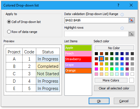
14042016 Go to Format. The list shows valid values the user can select simply press with left mouse button on a value with the mouse or use updown arrow keys. If you check Row of data range in the Apply to section you need to select the row range.
Under Allow List and enter a followed by the name of the list in the Source field. The drop down list that I use was created from cells that have the colors already in the word but I do not know how to make the list show the colors so it puts the word. Select a cell in which you want the dropdown to appear D3 in our case.
First we select the cell where we want the drop down to. Select Specific Text from the first dropdown list and containing from the 2nd drop-down list and specify the cell C1 in the textbox to specify that we are setting the color for the cell if the value is Apple. Click on the Format button and choose the color that you to apply for this value.
On the Data tab in the Data Tools group click Data Validation. To do this click a cell and go to Data. 29032013 Activate the Fill tab and specify the desired color.
In the New Formatting Rule dialog we will select. 09042021 Create the main drop down To make your primary drop-down list configure an Excel Data Validation rule in this way. How to Change the Background Color for Special Cells cells with formula errors or blanks In the Home tab we will go to the Styles group and click Conditional formatting Next we will select New Rule.
1 Check the scale you want to add color to in the Apply to section. We want to make a drop down list from the data contained in our list. This video explains how to create a data validation drop down list in Excel that changes the fill background andor font colour dependent on what is select.
Format the Excel Drop Down List. Tool button on the ribbon. A wizard box appears.
23082013 another from the drop down list it will change its color to a specified color. To create a drop down list where the background color depends on the text selected first create a drop down list in Excel using Data Validation then use Conditional Formatting to amend the background color. Now the conditional formatting of the color cells must be copied to the desired column.
In the source tab select the range of data for the drop-down list. You may wish to change the background color of the cell that contains the list or add a border to it so users can easily identify it. Select New rule from the list and a dialog box will appear.
In the Colored Drop-down list dialog box please do the following operations. Now click Home. Using the instructions from a previous Excel drop down list.
3 Click on Home. Repeat steps 4 through 10 for each option in the dropdown menus specifying the option in step 6 and choosing a different color in. 19082016 1 Click on cell with drop down list.
Creating a Drop Down List With Data Validation. In the Colored Drop-down list dialog do below settings. A Drop Down list lets you control what the user enters in a worksheet press with left mouse button on the black arrow next to the cell to expand the list.
4 Click Conditional Formatting in drop down list click the New Rule. Now every cell should have a dropdown with the names of the colors. This is how our new set of rules will look like.
The Data Validation window will pop up. How to Conditionally Formatting A Drop Down List. Fill then select a color of your choosing.
Then click Kutools. Under the Validation criteria select List. Color automatically in the drop down list to the cell with the drop down if that makes any.
Under Data Tab in the data tools section click on Data Validation. Select Specific Text option and select the cell for colour as in this case Red. Select the drop-down list cells then click Kutools.
In the settings under Allow click on Lists.
Get Organized With 2 Google Spreadsheets Features Skillcrush


Drop Down List In Excel In 2020 Data Validation Excel Tutorials Excel Shortcuts
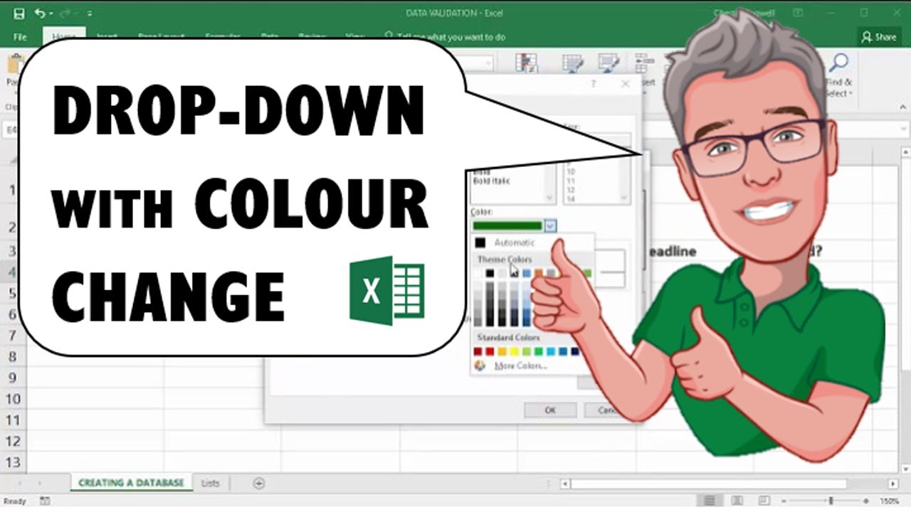
Excel Drop Down List Including Cell Colour Change Colour Fill Youtube
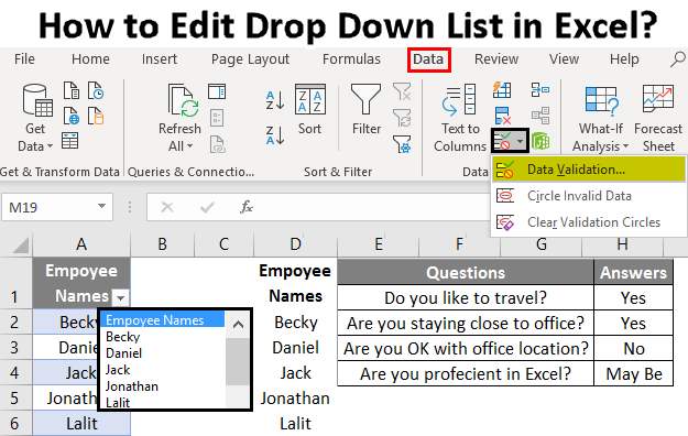
How To Edit Drop Down List In Excel Steps To Edit Drop Down List

How To Highlight Rows Based On Drop Down List In Excel
Get Organized With 2 Google Spreadsheets Features Skillcrush

How To Add Color To Drop Down List In Excel

Create Drop Down List In Excel With Color Tips Excel Drop Down List Force Users
Excel Drop Down List How To Create Edit And Remove Data Validation Lists


0 comments:
Post a Comment